论文阅读笔记-EPSILON An Efficient Planning System for Automated Vehicles in Highly Interactive Environments
[TOC]
本文为论文《EPSILON: An Efficient Planning System for Automated Vehicles in Highly Interactive Environments》的阅读后总结.
作者:Wenchao Ding,Lu Zhang 等
学校:香港科技大学
主题: 将预测和决策融合, 使用 POMDP 的概念包装决策树, 实现城市拥堵路段的自主换道. 局部轨迹规划可以参考他们之前的论文,解读博文链接.
论文网址: https://arxiv.org/pdf/2108.07993.pdf
开源地址: https://github.com/HKUST-Aerial-Robotics/EPSILON
I. INTRODUCTION
完成了两个层次的算法实现:a hierarchical structure with
- an interactive behavior planning layer, 通过 partially observable Markov decision process (POMDP) 解决
- an optimization-based motion planning layer, 通过 a spatio-temporal semantic corridor (SSC) to model the constraints posed by complex driving environments in a unified way. 通过优化算法解决, optimization-based scheme.
对于 POMDP 做的独特性开发是:
- The key to efficiency is guided branching in both the action space and observation space, which decomposes the original problem into a limited number of closed-loop policy evaluations.
- introduce a new driver model with a safety mechanism to overcome the risk induced by the potential imperfectness of prior knowledge.
批判的做法:
- pure geometry perspective, and adopted various rule-based or search-based techniques, which typically assume a behavior/trajectory prediction module is equipped on the system. 使用纯几何/基于规则的行为决策以及预测模型.
- The prediction is conducted independent of planning, and when the prediction is provided, the planner plans a trajectory with a sufficiently large safety margin. 预测与规划分离导致的规划总会留出富余的 margin 保证即便预测不准也不会产生问题. 因此把规划以及预测融合在一起更好. In cooperative and interactive scenarios, where this mutual influence is essential, coupled prediction and planning is more promising.
对于 Motion planning:
- 约束语义的统一编码化: All the constraints posed by complex semantics are encoded in a unified way using a spatio-temporal semantic corridor.
- 采用贝塞尔曲线作为轨迹输出: The piecewise B´ezier curve is adopted as trajectory parameterization for its convex hull and hodograph properties.
把决策与规划分离(decouple)的原因:After decoupling, the behavior planner only needs to reason about the future scenario at a relatively coarse resolution, while the motion planning layer works in the local solution space given the decision.
基于的研究是论文地址.
决策的上一篇论文地址,改进点在于不assumes other participants are rational, 而是 noisily rational,
其他亮点:
- 不单单在仿真上实现了还在实车上得到了验证.
- we extensively validate our system on a real automated vehicle in dense city traffic without an HD-map and purely relying on onboard sensor suites.
II. RELATED WORK
Behavior planning for automated vehicles
State-machine-based behavior planning
search-based methods
例如:A∗ graph search on a state lattice with static and dynamic events encoded as a cost map.
- an interactive multi-agent perspective(POMDPs), 问题在于 curse of dimensionality
- multiple policy decision making (MPDM),缺点: over-simplifies the action for the ego vehicle: each candidate policy contains only one semantic-
level action with a rather long duration, making MPDM a single-stage MDP.
- multiple policy decision making (MPDM),缺点: over-simplifies the action for the ego vehicle: each candidate policy contains only one semantic-
Motion planning for automated vehicles
- search-based methods based on the state lattice
- motion primitives
- optimization-based methods(本文的方法)
III. SYSTEM OVERVIEW
三层架构.
The output of perception is synchronized and fed to a semantic map manager module.其特点如下:
- is updated at 20 Hz.
- includes an occupancy grid for static obstacles, multiple tracklets for dynamic obstacles.
- road structures for lanes and traffic semantics.
Behavior planner consists of three processes: guided branching, scenario realization and evaluation.
scenario 的定义: incorporating a particular ego action sequence with a particular intention combination of other traffic participants.
The generated trajectory is fed to a trajectory server for re-planning scheduling, and the desired state for re-planning can be queried from the trajectory server.
IV. PROBLEM FORMULATION
notation:
$\mathcal{E}_t$ denote the ego-centric local environment at time t.
$x^i_t$ as the state of the vehicle $i ∈ V$ at time t,$i = 0$ is reserved for the ego vehicle.
$z_t$ observation received by ego agent.
$⟨z_t, \mathcal{E}_t⟩$ the input of the behavior planning layer.
$\mathcal{D}_t$ output is a decision, $\mathcal{D}_t := [x_{t+1}, x_{t+2}, . . . , x_{t+H}]$ for all agents, where $H$ denotes the planning horizon.$⟨\mathcal{D}_t, \mathcal{E}_t⟩$ input to the motion planning layer.
a tuple $⟨\mathcal{X},\mathcal{A}, \mathcal{Z}, T, O, R⟩$: POMDP model.
$\mathcal{X},\mathcal{A}, \mathcal{Z}$ are the state space, action space and observation space, respectively.
$T(x_{t−1}, a_t, x_t) = p(x_t|x_{t−1}, a_t)$ the probabilistic statet ransition model.
$O(x_t, z_t) = p(z_t|x_t)$ the observation model.
$R(x_{t−1}, a_t)$ is a real-valued reward function $R : \mathcal{X} ×\mathcal{A} → R$ for the agent taking a ction $a_t ∈ A$ in state $x_{t−1} ∈ \mathcal{X}$.
belief $b ∈ \mathcal{B}$, which is the probability distribution over $\mathcal{X}$.
$$
\begin{aligned}
b_{t}\left(x_{t}\right) &=p\left(x_{t} \mid z_{t}, a_{t}, b_{t-1}\right) \\
&=\eta O\left(x_{t}, z_{t}\right) \int_{x_{t-1} \in \mathcal{X}} T\left(x_{t-1}, a_{t}, x_{t}\right) b_{t-1}\left(x_{t-1}\right) d x_{t-1}
\end{aligned}
$$
where $η$ is a normalizing factor.
optimal policy $π^∗$ which maps the belief state to an action $π : B → A$, maximizing the expected total discounted reward over the planning horizon:
$$
\pi^{*}:=\underset{\pi}{\arg \max } \mathbb{E}\left[\sum_{t=t_{0}}^{t_{H}} \gamma^{t-t_{0}} R\left(x_{t}, \pi\left(b_{t}\right)\right) \mid b_{t_{0}}\right],
$$
$t_0$ the current planning time.
$γ ∈ [0, 1] $ a discount factor, 本文 $γ = 0.7$
an optimal policy is found by applying the Bellman equation on each internal node:
$$ \begin{aligned} V^{*}(b)=& \max _{a \in \mathcal{A}} Q^{*}(b, a) \\\\ =& \max _{a \in \mathcal{A}}\left\{\int_{x \in \mathcal{X}} b(x) R(x, a) d x\right.\\\\ +&\left.\gamma \int_{z \in \mathcal{Z}} p(z \mid b, a) V^{*}(\tau(b, a, z)) d z\right\} \end{aligned} $$ where $V^{*}(b)=\int_{s \in \mathcal{S}} V^{*}(s) b(s) d s$ is the optimal utility function for the belief state.$Q^∗(b, a)$ describes the optimal value of the belief-action pair.
一直搜索计算到 horizon, a complete trace $S_t =[b^∗_t , a^∗_{t+1}, z^∗_{t+1}, b^∗_{t+1}, ..., b^∗_{t+H}]$ on the belief tree by applying $$ \begin{aligned} a_{t}^{*} &=\underset{a_{t} \in \mathcal{A}}{\arg \max } Q^{*}\left(b_{t-1}, a_{t}\right) \\\\ z_{t}^{*} &=\underset{z_{t} \in \mathcal{Z}}{\arg \max } p\left(z_{t} \mid b_{t-1}, a_{t}^{*}\right) \end{aligned} $$
The final decision $D_t$ can be generated by simply applying $x_t = {\arg \max}_x b^∗_t (x)$ for each step in $\mathcal{S}_t$.
$x^i_t ∈ \mathcal{X}^i$ is the $i$-th vehicle’s state containing its position, velocity, acceleration, heading, and steering angle.
$a_t = a^0_t, \mathcal{A} = \mathcal{A}^0$ action of the original problem, 因为我们只能对自车的 throttle/brake and steering 控制, 其他车与 traffic participants 是被间接控制的.
同上 $p(x_t|x_{t−1}, a_t) = p(x^0_t, …, x^N_t |x^0_{t−1}, …, x^N_{t−1}, a^0_t)$: The complete state transition model $T$ can be represented as a joint distribution.
assume that the instantaneous transitions of each vehicle are independent, resulting in:
$$ \begin{aligned} & p\left(x_{t} \mid x_{t-1}, a_{t}\right) \\\\ \approx & \underbrace{p\left(x_{t}^{0} \mid x_{t-1}^{0}, a_{t}^{0}\right)}_{\text {ego transition }} \prod_{i=1}^{N} \int_{\mathcal{A}^{i}} \underbrace{p\left(x_{t}^{i} \mid x_{t-1}^{i}, a_{t}^{i}\right)}_{i \text {-th agent's transition }} \underbrace{p\left(a_{t}^{i} \mid x_{t-1}\right)}_{\text {driver model }} d a_{t}^{i}, \end{aligned} $$$p(x_i^t|x^i_{t−1}, a^i_t)$ is the assumed transition model of the other agents that reflects the agent’s low-level kinematics.
$p(a^i_t|x_{t−1})$ is the assumed driver model representing the high-level decision process of the other agents.
assuming the observation processes are independent: $p\left(z_{t} \mid x_{t}\right)=\prod_{i=0}^{N} p\left(z_{t}^{i} \mid x_{t}^{i}\right)$.$z^0_t = z_t$ : position and velocities of other vehicles generated by the perception module.
belief 公式可以化为:
$$
b_{t}\left(x_{t}\right)=\eta \cdot \overbrace{p\left(z_{t}^{0} \mid x_{t}^{i}\right) \int_{\mathcal{X}^{0}} p\left(x_{t}^{0} \mid x_{t-1}^{0}, a_{t}^{0}\right) b_{t-1}^{0}\left(x_{t-1}^{0}\right) d x_{t-1}^{0}}^{\text {belief update for ego car agent }} \quad \prod_{i=1}^{N} \overbrace{p\left(z_{t}^{i} \mid x_{t}^{i}\right) \int_{\mathcal{X}^{i}} \int_{\mathcal{A}^{i}} p\left(x_{t}^{i} \mid x_{t-1}^{i}, a_{t}^{i}\right) p\left(a_{t}^{i} \mid x_{t-1}\right) b_{t-1}^{i}\left(x_{t-1}^{i}\right) d a_{t}^{i} d x_{t-1}^{i}}^{\text {belief update for other agents }} .
$$
问题: 既然都是独立的那么怎么体现 interactive process 呢?
although the state transitions of each agent in each step are independent, the assumed driver models $p(a^i_t|x_{t−1})$ and observation models $p(z^i_t|x^i_
t)$ leverage all agents’ states and observations, making the belief update an interactive process.
Belief update using observations, which is exactly the role of behavior prediction.
the role of the motion planning boils down to a local trajectory optimization problem, 规划仅仅成为 local optimization 问题.
V. EFFICIENT BEHAVIOR PLANNING
A. Motivating Example
对 action 进行剪枝: only a few long-term semantic-level actions given common driving knowledge (e.g., lane keeping, yielding, overtaking, etc.).
说的冠冕堂皇一点的话: mimic the decision-making process of human drivers and utilize domain knowledge for efficient exploration.
three discretized longitudinal velocities and three lateral accelerations 就会导致灰色的巨多的 tree, 但是按照驾驶语义的化, 只需按照紫色线寻找.
总结成三点:
- Flexible driving policy:Compared to MPDM, the proposed method considers multiple future decision points rather than using a single semantic action in the whole planning horizon. 搜索时不止用一个 action.
- Efficient policy evaluation: pick out the potentially risky scenarios conditioned on the ego policy to reduce computational expense during the policy evaluation. 两个字:剪枝.
- Enhanced risk handling in real traffic: with a safety mechanism, 有紧急安全备案.
B. Guided Action Branching
$\phi_{t}^{i} \in \Phi^{i}$: represents the semantic action for agent $i$ at time $t$, $\Phi^{i}$ 时 action set, can be different depending on the agent type.
discrete semantic-level actions ${K, L, R}$, denoting “keep lane”, “left lane change” and “right lane change”, respectively.
因此动作的概率计算变为了 $p(a^i_t|x_{t−1}, φ^i_t)$.
私认为这不就是应用 MDP 的 action space 离散化过程吗? 这不是理所应当的吗?搞得这么复杂….另外使用 semantic-level actions 不还是基于规则的吗, 只不过把规则变成了分支然后去搜索. 创造新名词: domain- specific closed-loop policy tree (DCP-Tree).
Update@20220626: 此处的认识不足, 在自学《编译原理》后, 发现作者们的思路没有问题, 使用语义决策树, 是很自然的, 值得学习. 希望越来越多的认知被打破!
$$ \begin{array}{r} p\left(x_{t} \mid x_{t-1}, \phi_{t}\right) \approx \int_{\mathcal{A}^{0}} \underbrace{p\left(x_{t}^{0} \mid x_{t-1}^{0}, a_{t}^{0}\right)}_{\text {ego state transition }} \underbrace{p\left(a_{t}^{0} \mid x_{t-1}, \phi_{t}^{0}\right)}_{\text {ego controller }} d a_{t}^{0} \\\\ \prod_{i=1}^{N} \int_{\mathcal{A}^{i}} \underbrace{p\left(x_{t}^{i} \mid x_{t-1}^{i}, a_{t}^{i}\right)}_{i \text {-th agent's transition }} \underbrace{p\left(a_{t}^{i} \mid x_{t-1}\right)}_{\text {driver model }} d a_{t}^{i} . \end{array} $$ 其中: $$ p\left(a_{t}^{i} \mid x_{t-1}\right)=\sum_{\phi_{t}^{i} \in \Phi^{i}} \underbrace{p\left(a_{t}^{i} \mid x_{t-1}, \phi_{t}^{i}\right)}_{\text {agent controller }} \underbrace{p\left(\phi_{t}^{i} \mid x_{t-1}\right)}_{\text {new driver model }} $$ $p\left(\phi_{t}^{i} \mid x_{t-1}\right)$ reflects the **decision process** of the the $i$-th agent.剪枝的另一个思路: as human drivers, we typically do not change the driving policy back and forth in a single decision cycle. Therefore, from the ongoing action, each policy sequence will contain at most one change of action in one planning cycle. 动作的持续性.
the size of the leaf nodes in the DCP-Tree is $O[(|A|−1)(h−1)+1], ∀h > 1$
C. Guided Observation Branching
改进 Monte Carlo-based method:
assume the ego state $x^0_t$ is fully observable and the observations $z_t$ (i.e. tracklets) are noise-free.
$p(φ^i_t|x_{t−1})$ 直接单因素决定, semantic action is fully determined by the hidden states, such as intention.
$p(x^i_t|x^i_{t−1}, a^i_t)$ no control noise.
hidden states of other agents are not updated in the forward simulation, which means that the semantic actions of other agents are fixed. 也就是$φ^{i \ne 0}_t$ only depends on the initial belief $b_t^0$.原因: 1是计算资源,2是实战觉得效果可以.
the total utility of the policy is the weighted sum of the sampled scenarios, while the weights are exactly the value of the initial belief.
the semantic action for the other agent is represented by the action of pursuing a particular center-line. 这样就把他车的行为概率坍塌到了追寻不同车道中心线的概率.至于概率分布使用自建的 learning-based intention estimator 确定.
Since each traffic participant potentially has multiple choices (e.g., multiple candidate center-lines), we define one combination of intentions for all the traffic participants as one scenario.
scenario的组合太多怎么办?
conditional focused branching (CFB)
attention of the human driver for nearby vehicles is biased differently when intending to conduct different maneuvers. 针对不同的 action 对 scenarios 进行剪枝.
图解如下: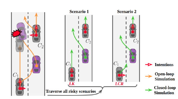
由于 $C_1$ 风险较大,会展开所有 intention 可能性, 但是对于跟车对象的 $C_2$ 风险没那么大, 只对其展开概率最大的分支.
D. Multi-agent Forward Simulation
simple model-based driver model by using the intelligent driver model (IDM) for velocity control and pure pursuit for steering control.
对于自车则使用较正常的 model:context-aware controller,contains a velocity controller and a steering controller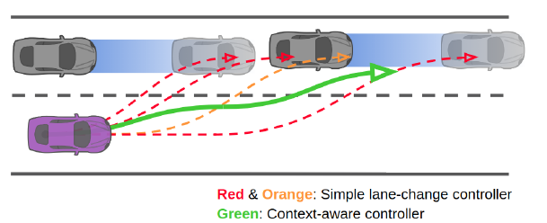 .
.
说白了,其实就是混用成熟的 action set 实现策略, 代替简单的单一的 action 策略, 进行剪枝.
E. Safety Mechanism
In traditional methods, this issue is dealt with by leaving sufficiently large safety margins.
- embedding a safety module in the context-aware controller, responsibility-sensitive safety (RSS).
- setting the safety criterion in the policy selection, backup plan(例如回撤 policy).
- 最坏的情况下 If there are no safe policies at all, meaning that the behavior planning has failed, a warning signal will be displayed, and the low-level active protection, such as autonomous emergency braking (AEB), will be triggered.
RSS 具体执行过程(三层监控):
For each simulation step, we check whether the simulated state for the controlled vehicle is RSS-safe. If not, we check whether the control signal provided by the context-aware controller follows the criterion of proper response defined by the RSS model. If still not, we generate a safe control signal obeying the proper response and override the control output.
F. Policy Selection
The reward function consists of three parts:
- efficiency
- safety
- navigation
并行计算的部分:
- Evaluation for each policy sequence
- forward simulation
整体决策算法过程如下: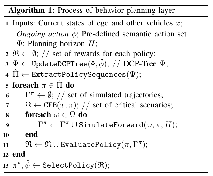
VI.TRAJECTORY GENERATION WITH SPATIO-TEMPORAL SEMANTIC CORRIDOR
对规划模块而言,决策部分给出的结果不一定可以严格执行,因此有必要使用代价函数来约束规划模块的轨迹生成. 代价函数由2部分组成:
- smoothness cost
- similarity cost(与决策给出结果的差异)
代价函数如下:
the cost $J_j^σ$ of the $j$-th segment on dimension $σ$:
$$
\begin{aligned}
J_{j}^{\sigma}=w_{s}^{\sigma} \cdot \int_{t_{j-1}}^{t_{j}} &\left(\frac{d^{3} f_{j}^{\sigma}(t)}{d t^{3}}\right)^{2} d t +
w_{f}^{\sigma} \cdot \frac{1}{n_{j}} \sum_{k=0}^{n_{j}}\left(f_{j}^{\sigma}\left(t_{k}\right)-r_{j k}^{\sigma}\right)^{2}
\end{aligned}
$$
$w_s^σ$ and $w_f^σ$ denote the weight for the smoothness cost and the similarity cost.
$r_{jk}^σ$ denotes the $k$-th reference state on dimension $σ$,generated by the ego-simulated states corresponding to the $j$-th segment.
$t_k$ is the timestamp of $r_{jk}^σ$.
$n_j$ the number of reference states in the $j$-th segment is determined by the result of cube inflation.
写成矩阵形式:
$$ \begin{aligned} J_{j}^{\sigma} &=\mathbf{p}_{j}^{\mathrm{T}}\left(w_{s}^{\sigma} \mathbf{Q}_{s}+w_{f}^{\sigma} \mathbf{Q}_{f}\right) \mathbf{p}_{j}+w_{f}^{\sigma} \mathbf{c}^{\mathrm{T}} \mathbf{p}_{j} \\\\ &=\frac{1}{2} \mathbf{p}_{j}^{\mathrm{T}} \hat{\mathbf{Q}} \mathbf{p}_{j}+\hat{\mathbf{c}}^{\mathrm{T}} \mathbf{p}_{j} \end{aligned} $$$Q_s$ and $Q_f$ are real symmetric matrices related to the
smoothness term and similarity term.
$c$ is a real vector.
最终规划变为一个 quadratic programming (QP) 问题,使用 OOQP 求解器求解.
VII. IMPLEMENTATION DETAILS
A. Semantic-level Actions and DCP-Tree
- the lateral action set can be defined as the target center-line $c_i$ of the adjacent lanes. The number of lateral actions $N_a^{lat}$ in the set is conditioned on the driving context since the adjacent lanes may be unavailable (due to traffic rules) or just not exist.
- predefined velocity controller rather than directly applying longitudinal acceleration signals. longitudinal semantic action set with $N_a^{lon} = 3$ items: ${Aggressive, Moderate, Conservative}$.
- DCP-Tree, depth = 5.
- each semantic-level action time duration = 1s
- closed-loop simulation: 0.2s
- planning horizon: 5s
B. Context-aware Forward Simulation Model
基于 frenet 坐标系:
curvilinear coordinate frame, where $s(·)$ and $d(·)$ denote the longitudinal and lateral positions in the path-relative coordinate frame.
例如:
- lane keeping: lateral controller = pure pursuit controller + longitudinal motion = IDM
- lane changing: lateral controller = the reactive pure pursuit, longitudinal controller = gap-informed velocity controller.
对于横向 reactive lateral motion controller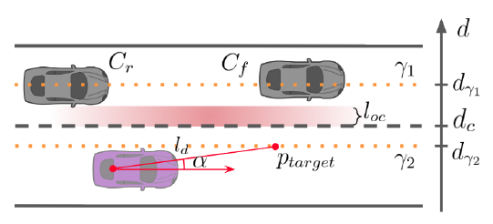
分为2种情况:
- 相邻车道是安全的(例如空的),直接把横向控制的终点设置在相邻车道的 $\gamma_1$处.
- 相邻车道不是足够安全的,先在当前车道靠近相邻车道等时机成熟再换过去,也就是两个层级,先靠近 $\gamma_2$,再靠近 $\gamma_1$.
$p_{target}$ 为预瞄点, $l_{oc}$ 为安全 buffer.
$$
d_{γ_2} = d_c − \frac{W_{ego}}{2} - \max(0, l_{safe} − l_{oc}),
$$
corresponding steering angle can be calculated using the pure pursuit controller $δ_{ctrl} = \arctan \frac{2L sin α}{l_d}$.
对于纵向 gap-informed longitudinal motion controller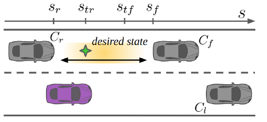
下面上面带点的符号均为速度:
期待的结果$[s_{des} , ṡ_{des} ]$
$$ s_{des} = \min(\max(s_{tr} , s_{ego}), s_{tf} ) \\\\ ṡ_{des} = \min(\max(ṡ_r , ṡ_{pref} ), ṡ_f ), $$ where $[ṡ_r , ṡ_f ]$: the observed longitudinal velocity of $C_r$ and $C_f$ $ṡ_{pref}$: the preferred longitudinal cruise velocity assigned by user and traffic rules $s_{tr}$ and $s_{tf}$:the threshold positions derived from the time headway corresponding to $C_r$ and $C_f$. $$ \begin{aligned} \left[\begin{array}{c} s_{t r} \\\\ s_{t f} \end{array}\right]=\left[\begin{array}{c} s_{r}+l_{\min }+T_{s a f e} \dot{s}_{r} \\\\ s_{f}-l_{\min }+T_{s a f e} \dot{s}_{e g o} \end{array}\right] \end{aligned} $$ where $l_{min}$ and $T_{safe}$ are the minimum spacing and safe time headway.根据上面的状态推导应用如下 PD 控制器:
$$
\begin{aligned}
a_{track} = K_v (ṡ_{des} + K_s(s_{des} − s_{ego}) − ṡ_{ego})
\end{aligned}
$$
同时考虑到还有跟车的可能通过 IDM 模型算出 $a_{idm}$,最终 $a$ 的结果为:
$$
\begin{aligned}
a_{ctrl} := \min(a_{track} , a_{idm} )
\end{aligned}
$$
最终 check output $[δ_{ctr},a_{ctrl}]$ 是否 RSS proper response.
下表为上面横纵向的变量一览表.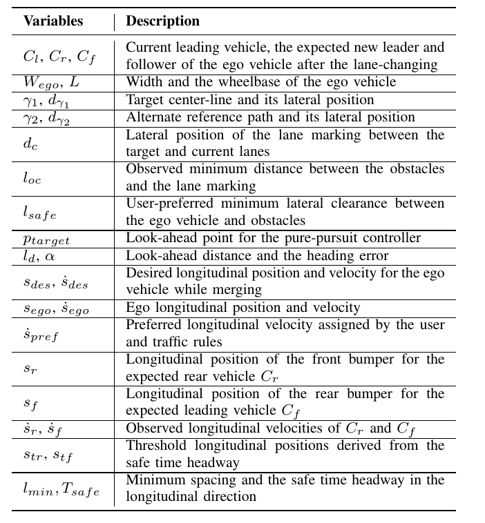
transition model $p(x^i_t|x^i_{t−1}, a^i_t)$, all agents are described using the kinematic bicycle model.
C. Intention Estimator
a neural network-based method to estimate the intention of the surrounding agents using the observation history and environmental information.
整体结构如下: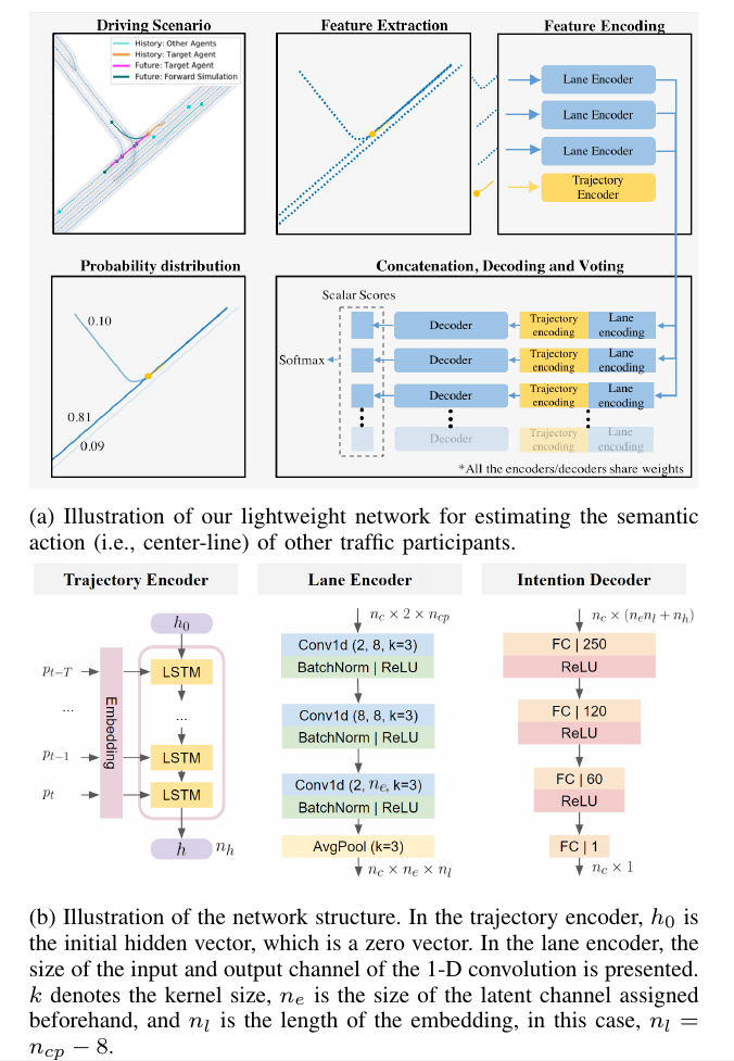
D. Policy Evaluation
$$
F_{total} = λ_1 F_e + λ_2 F_s + λ_3 F_n = − R,
$$
$F_e$: efficiency cost
$F_s$: safety cost
$F_n$: navigation cost
$F_e$: efficiency cost
$$
F_{e}=\sum_{i=0}^{N_{a}} F_{e}^{i}=\sum_{i=0}^{N_{a}}\left(\lambda_{e}^{p} \Delta v_{p}+\lambda_{e}^{o} \Delta v_{o}+\lambda_{e}^{l} \Delta v_{l}\right)
$$
$∆v_p = |v_{ego} − v_{pref} |$, velocity difference between the current simulated velocity and the preferred velocity for the ego vehicle.
$∆v_o = \max(v_{ego} − v_{lead}, 0)$, $v_{lead}$: speed of leading vehicle.
$∆v_l = |v_{lead} − v_{pref} |$
$N_a$ is the number of semantic actions in a policy.
$F_s$: safety cost
$$
\begin{aligned}
F_{s} &=\lambda_{s}^{c} b_{\mathrm{c}}+\sum_{i=0}^{N_{s}} b_{\mathrm{r}} F_{s}^{i} \\
&=\lambda_{s}^{c} b_{\mathrm{c}}+\sum_{i=0}^{N_{s}} b_{\mathrm{r}} v_{e g o} \lambda_{s}^{r 1} e^{\lambda_{s}^{r 2}\left|v_{e g o}-\min \left(\max \left(v_{e g o}, v_{r s s}^{l b}\right), v_{r s s}^{u b}\right)\right|}
\end{aligned}
$$
where
$b_c$ and $b_r$: the boolean values denoting the collision and the violation of RSS-safety for the ego simulated state.
$λ^c_s$ is the penalty for collision.
$N_s$: the total number of the simulated states in the ego trajectory.
The cost for RSS-dangerous is designed in an exponential form to emphasize the degree of the RSS-safety violation.
$λ^{r1}_s$ and $λ^{r2}_s$: tunable parameters.
$F_n$: navigation cost
取决于2个方面的因素: user preference(HMI,例如指令换道) and decision context(decision consistency).
$$
F_{n}=\lambda_{n}^{u s e r} b_{n a v i}+\lambda^{c o n s i s t} b_{c o n s i s t}
$$
VIII. EXPERIMENTAL RESULTS
A. Quantitative Analysis
Semantic-level action and forward simulation
预测与决策的融合是否会导致 over-simplifies the problem and results in significant loss in the fidelity of future anticipation?
通过 benchmark 验证: two state-of-the-art learning-based trajectory prediction techniques, namely, TPNet and UST .
Dataset: Argoverse motion forecasting dataset
Training: Pytorch + a single NVIDIA GTX 1080 GPU + Adam optimizer with a batch size of 128. initiate the learning
rate to 1e-3 and decay to 1e-4 after 35 epochs. The total time cost is around 3 hours for 50 epochs.
Metrics: Average displacement error (ADE) and final displacement error (FDE) + Minimum over N (MoN) metrics such as minADE
and minFDE.
Baselines: whether map information or prior knowledge is used, TPNet has several variants.
- Nearest Neighbor (NN)
- LSTM Encoder-Decoder network
- TPNet with only 2-second past observations and without road map information
- TPNet with road map information as input
- TPNet with prior knowledge for constraining proposals.
- TPNet with prior knowledge for generating multiple proposals.
- UST: Unified spatio-temporal representation
Results:
- one trajectory hypothesis: > NN and LSTM ED, but < TPNet and UST
- multiple prediction hypotheses: > all baselines
- impact of the accuracy of intention estimation on the scenario realization: BIG! 不可省略
- may explore using learning-based controllers for the forward simulation
Impact of coupling prediction and planning
构造了一个专门的场景: 前车突然刹停,自车必须瞅准时机换道提升行驶效率,这时候对自车要求较高,不仅要考虑周围环境还要考虑自车突然换道对相邻车道后车的交互性.
对周围 AI 车辆的模拟策略:
- The policy for AI agents is a simple adaptive cruising policy adapted from the intelligent driver model.
- aggressiveness levels: adjusting the desired time headway that directly determines the longitudinal distance to the leading vehicle.
- cooperative range(friendliness): yield and keep distance to the cut-in vehicle
Metrics:
- safety: RSS
- travel efficiency: avoid waiting indefinitely in the hazard
every planning cycle and calculate the average. 15 seconds to safely pass the hazard.
Baseline:independent trajectory prediction module, derived from multi-agent forward simulation, but exclude the decision of the controlled vehicle.
Results: when increasing the aggressiveness, decoupled prediction-planning failed.
Impact of the safety mechanism
Baseline: excludes the safety mechanism
benchmark scenario and metrics are the same as those in the previous section.
Results:in aggressive and less cooperative traffic, baseline is not good.
Analysis: EPSILON w/o safety always assumes the following vehicle in the nearby lane will yield
图解如下:
Computation Time Cost
硬件: Intel i7-8700 with 32GB RAM
分析方法: 250 frames for statistical analysis
结果:
motion planner is basically constant
two modules is all restricted within 50 milliseconds
B. Qualitative Analysis
实车测试系统架构: two sets of forward-facing stereo cameras, four fish-eye cameras, four millimeter-wave radars, six ultrasonic sensor and a low-cost INS. a single NVIDIA Xavier with an 8-core ARM-base CPU.
control system is based on the model predictive control (MPC)
实车测试环境: four-lane dual carriageway with a speed limit of 80 km/h
结果:
- overall success rate for lane-changing (over 80%)
- human-like maneuvers such as “find gap then merge” and cut-in handling can be achieved automatically.
- 第三次成功率降到了 65%, 就开始甩锅了…
- miles per intervention (MPI) 无法评价本系统,因为本系统可以调成纯保守型的,那么根本不会有接管.那如何评价系统表现呢?用复杂场景解决能力,下面提出了四种场景.
- Intelligent gap finding and merging, 指令换道
- Interaction-aware overtaking,指令加速换道
- Low-speed automatic lane change in dense traffic,自动连续换道,即便换道过程中后车信息不准
- Cut-in handling and automatic lane change 被他车 cut in 后自动换道
阅后小结
- 最大的算法概念 POMDP 并没有使用强化学习常规的 Monte-Carlo, DP 等算法求解, 还是只是考虑输入概率分布的决策树而已, 然后再进行 search 找到最优解得到决策. 有点借概念包装的感觉. MDP 我觉得最具挑战的的确是如何把连续的函数离散成可求解的离散空间, 但是最终的求解 forward-simulation 居然是定长的,而不是设置吸收态,没法算下去的 episode branch 早点退出节省资源.
- 值得借鉴的点还是不少的, 例如 grid map 下障碍物的数据格式的处理, forward-simulation 中预测他车与自车轨迹(state)的 motion module 的建立, 使用 RSS “标准” 进行安全性 backup 等.
- 源码的架构还是很清晰的, 可读性不差.
论文阅读笔记-EPSILON An Efficient Planning System for Automated Vehicles in Highly Interactive Environments
